In today's blog, I will present the Fundamental Theorem of Symmetric Polynomials. In my
previous blog, I talked about
symmetric polynomials and
elementary symmetric polynomials. In today's blog, I show the relationship between the two.
The content in today's blog is taken straight from Harold M. Edwards'
Galois Theory.
Theorem 1: Fundamental Theorem on Symmetric PolynomialsEvery
symmetric polynomial in
r1, ..., rn can be expressed as a polynomial in
elementary symmetric polynomials σ1, ..., σn. In addition, a symmetric polynomial with integer coefficients can be expressed as a polynomial in elementary symmetric polynomials with integer coefficients.
Proof:
(1) For
n=1, the
symmetric polynomial is
x - r1 so that we see that
a1 = -r1 and
σi = (-1)1(-r1)=r1 [See Definition 1,
here for definition of
symmetric polynomial; see Definition 2,
here for definition of the
kth elementary symmetric polynomial]
(2) if
a1 is an integer, then
r1 is an integer and
σ1 is an integer.
(3) The polynomial in elementary symmetric functions is then
x - σ1 which shows that the theorem is true for
n=1.
(4) Let's assume that the theorem has been proved for all symmetric polynomials up to
n-1.
(5) Let
G(r1, r2, ..., rn) be a
symmetric polynomial in
n variables so that:
G(r1, r2, ..., rn) = (x - r1)*(x - r2)*...*(x - rn)(6) Let
Gi be a series of polynomials such that:
G(r1, r2, ..., rn) = G0 + G1rn + G2(rn)2 + ... + Gv(rn)vwhere:
v is the highest power of
rn that occurs in
G and each
Gi is only made up of
r1, r2, ..., rn-1.
We can see that
G0 is a polynomial that doesn't include
rn.
G1 includes all multiples of
(rn)1.
G2 includes all the multiples of
(rn)2 and so on up until
v which is defined as the highest power of
rn which can be
1.
(7) Now, since
G(r1, r2, ..., rn) is a
symmetric polynomial, it is unchanged if any two variables
ri and
rj are interchanged. [See Definition 1
here for definition of
symmetric polynomial]
(8) Since
G(r1, r2, ..., rn) is unchanged with any interchange, so too are the polynomials defined by
Gi are unchanged.
(9) This means that each
Gi is itself a
symmetrical polynomial on
r1, r2 ... rn-1.
(10) By the inductive hypothesis in step #4, we can assume that each
Gi is itself expressible as an
elementary symmetric polynomial in
r1, r2, ..., rn-1(11) Let
τi, τ2, ..., τn-1 denote these
elementary polynomials in
(n-1) variables such that [See Definition 2
here for definition of
elementary symmetric polynomials]:
τ1 = r1 + r2 + ... + rn-1τ2 = r1r2 + r1r3 + ... + rn-2rn-1...τn-1 = r1r2*...*rn-1 [NOTE: Each
τi represents the sum of all
i-combinations of
1 ... n-1. So,
τ1 is the sum of all
1-combinations,
τ2 is the sum of all
2-combinations, and
τn-1 is the sum of all
n-1 combinations (for which there is only one)].
(12) So, from the inductive hypothesis, if we let
Gi(r1, ..., rn-1) represent the
symmetric polynomial Gi, we can see that there exists another polynomial
gi such that:
Gi(r1, ..., rn-1) = gi(τ1, τ2, ..., τn-1)(13) Further, from the inductive hypothesis, we know that if
Gi has integer coefficients, then, so does
gi.
(14) Let
σ1, σ2, ..., σn be the
elementary symmetric polynomials in
n variables.
(15) We can now restate
σi in terms of
τi since:
σ1 = r1 + r2 + ... + rn = τ1 + rn
σ2 = r1r2 + r1r3 + ... + rn-1rn = τ2 + rnτ1[Note:
rn*τ1 is equal to the sum of all
(n-1) 1-combinations with
rn]
σ3 = r1r2r3 + r1r2r4 + ... + rn-2rn-1rn = τ3 + rnτ2
[Note:
rn*τ1 is equal to the sum of all
(n-1) 2-combinations with
rn]
σ4 = τ4 + rnτ3...σn = r1*r2*....*rn = 0 + rn*tn-1[Note: the main idea here is the
σi represents the sum of all
i-combinations of
n variables. We are now equating these sums with
τi which represents the sum of all
i-combinations of
(n-1) variables. In other words, we are now including the new combinations with r
n.]
(16) We can now restate the equations in step #15 in terms of
τi to get (using the basic algebraic operations of addition/subtraction to both sides of the equation):
τ1 = σ1 - rnτ2 = σ2 - rnτ1 = σ2 - rn(σ1 - rn) = σ2 - rnσ1 + (rn)2τ3 = σ3 - rnτ2 = σ3 - rnσ2 + (rn)2σ1 - (rn)3....τn-1 = σn-1 - rnτn-2 = σn-1 - rnσn-2 + ... + (-1)n-1(rn)n-1(17) Finally, we can use the last equation in step #15, to get:
0 = σn - rnτn-1 = σn - rnσn-1 + ... + (-1)n(rn)n. (18) Since we restate all the terms
τi in terms of
rn and
σi, we can define a polynomial
fi(σ1, σ2, ..., σn-1), such that using step # 12, we have:
G(r1, r2, ..., rn) = f0 + f1(σn) + f2(σn)2 + ... + fμ(σn)μwhere each
fi is a polynomial strictly in terms of
σ1, σ2, ..., σn-1 and does not include
σn.(19) Each
fi has integer coefficients if
G does since:
(a) Using steps #16, we can state each
fi in terms of
τ1,...,τn-1(b) From step #13, we know that
τ1,...,τn-1 have integer coefficients if
G has.
(20) From step #17, we get the following:
(rn)n = (rn)n-1σ1 - (rn)n-2σ2 + (rn)n-3σ3 + ... + (-1)n-1σn(21) If
μ ≥ n, then we can continuously apply the result in step #18 to the result in step #20, to get:
G(r1, r2, ..., rn) = f0(σ) + f1(σ)rn + f2(σ)(rn)2 + ... + fn-1(σ)(rn)n-1(22) Since interchanging any values
ri with
rj doesn't change the value of
G(r1, r2, ..., rn), then it doesn't change the value of
f0(σ) + f1(σ)rn + f2(σ)(rn)2 + ... + fn-1(σ)(rn)n-1(23) By repeatedly interchanging distinct
ri and
rj values where
i ≠ j, we get the following
n set of equations using step #21:
G(r1, r2, ..., rn) = f0 + f1r1 + f2(r1)2 + ... + fn-1(r1)n-1
G(r1, r2, ..., rn) = f0 + f1r2 + f2(r2)2 + ... + fn-1(r2)n-1
...
G(r1, r2, ..., rn) = f0 + f1rn + f2(rn)2 + ... + fn-1(rn)n-1(24) We can think of these
n equations of
n terms as an
n x n matrix of the form
(ri)j-1 where
i = the column
(1 ... n) and
j = the row
(1 ... n).
(25) The determinant of this matrix which is a polynomial in
r1, r2, ..., rn is nonzero since this is an example of the transpose of the Vandermonde Matrix [see Definition 1,
here] and:
(a) From the properties of determinants, we know that
det(Vn) = det(VnT) [See Theorem 9,
here]
(b) The formula for the
determinant of the Vandermonde matrix is (see Theorem 1,
here):


(c) Since by assumption
r1 ≠ r2 ≠ ... ≠ rn [since each of the parameters is distinct], we can conclude that
det(Vn) ≠ 0.
(26) We can think of the set of equations as a multiplication between the above matrix
[(ri)j-1] and the vector [f
0(σ), f1(σ), ..., fn-1(σ)] [See
here for review of matrix multiplication] since:


(27) But, the the set of equations is also the result of multiplying the vector
[G,0,0,...,0] since:
(a) We have the following equation:
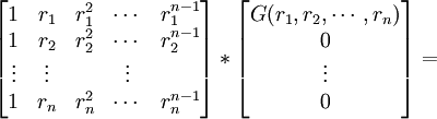

(b) From step #23, we have:
=
(c) So we can conclude that the following two equations are equal:

(28) Since the determinant in step #24 above is nonzero, the matrix is
invertible (see Theorem 4,
here) and we can multiply its inverse to both sides to get:

(29) From this, we can conclude that:
f0 = G and
f1=0, ..., fn-1=0. [See Definition 2,
here]
(30) Since
f0 is an
elementary symmetric polynomial (see step #18 above) and since
f0 has integer coefficients if
G does (see step #19 above), the conclusion follows from mathematical induction (see
here for review of mathematical induction).
QED
In my
next blog, I will complete the proof by reviewing the formula for the determinant of the Vandermonde Matrix. In a future blog, I will show how this theorem can be used to derive Newton's identities.
References


