The Zeta Function for Cyclotomic Integers

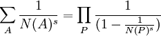
To get to the Kummer class formula, it is necessary to establish a zeta function for cyclotomic integers:



where A ranges over the set of ideal numbers, P ranges over the set of prime divisors of ideal numbers, and N(X) is the norm for these ideal numbers [for review of ideal numbers, start here] and s is greater than 1.

The content in today's blog is taken from Harold M. Edwards' Fermat's Last Theorem: A Genetic Introduction to Algebraic Number Theory.

Theorem 1: For s greater than 1, ∏ (1 - N(P)^-s)^-1 converges absolutely

Proof:

(1) Let λ be a prime number such that α^λ = 1 for any positive integer i less than λ, αⁱ ≠ 1. [See here for review of cyclotomic integers and λ]

(2) N(P) = p^f where p is a prime divisible by the prime divisor P and f is the exponent of p mod λ (or f=1 if p = λ) [See Lemma 1, here for proof N(P)=p^f or here for f=1 if p=λ]

(3) N(P)^-s = p^-fs ≤ p^-s

(4) Let e = (λ - 1)/f [See Lemma 1, here for proof that f divides λ-1] so that e ≤ λ - 1.

(5) We know from a previous result (see Lemma 1, here), that there are e prime divisors for a given prime p so that we know that:

∑ N(P) for a given P ≤ (λ - 1)∑ p^f

(6) So that:

∑ N(P)^-s ≤ (λ - 1) ∑ p^-fs which is less than (λ - 1)∑ p^-s which is less than (λ - 1)∑ n^-s

(7) From a previous result (see Theorem 1, here), we know that ∑ n^-s converges if s is greater than 1 so, we can conclude that ∑ N(P)^-s necessarily converges.

(8) Since N(P)=p^f is greater than 0, it follows that ∑ N(P)^-s = ∑ abs(N(P)^-s) and using Lemma 3, here, we can conclude that:

∏ (1 - abs(N(P)^-s)) converges

(9) This gives us (see Definition 1, here) that ∏ (1 - N(P)^-s) converges absolutely.

(10) Using the Reciprocal Law (see Lemma 6, here), we conclude that ∏ (1 - N(P)^-s)^-1 also converges absolutely.

QED

Lemma 2: For s greater than 1, ∑ N(A)^-s ≤ ∏ (1 - N(P)^-s)^-1

Proof:

(1) Let A* be any set of A and S* be defined such that S* = ∑ (A ∈ A*) N(A)^-s

(2) Let P* be the set of prime divisors that make up any of the A in A*. [See here for a review of prime divisors of an ideal number]

(3) For each P ∈ P*, we see that (1 - N(P)^-s)^-1 = 1 + N(P)^-s + N(P²)^-s + N(P³)^-s + .... [ See Lemma 1, here]

(4) It is then clear that ∏ (1 - N(P)^-s)^-1 = the product of all of these geometric series which includes all A in A*.

(5) Since N(Pⁱ) ^-s continues ad infinitum, there also necessarily exists N(Pⁱ)^-s that is not a divisor of any N(A) where A ∈ A* since A* is a finite set by assumption.

(6) So, any partial sum is less than the partial product.

(7) In this way, we can conclude that the infinite sum ∑ N(A) ≤ the infinite product ∏ (1 - N(P)^-s)^-1

QED

Corollary 2.1: ∑ N(A)^-s converges absolutely.

Proof:

(1) By Lemma 2 above, ∑ N(A)^-s ≤ ∏ (1 - N(P)^-s)^-1.

(2) Since ∏ (1 - N(P)^-s)^-1 converges (see Theorem 1 above), then ∑ N(A)^-s necessarily converges too.

(3) Since all values N(A)^-s are positive, it follows that ∑ N(A)^-s converges absolutely. (see Definition 2, here)

QED

Theorem 3: ∑ N(A)^-s = ∏ (1 - N(P)^-s)^-1

Proof:

(1) By Lemma 2 above, we have:

∑ N(A)^-s ≤ ∏ (1 - N(P)^-s)^-1

(2) Let P* be the same set of prime divisors from Lemma 2 above.

(3) It is clear that ∏ (1 - N(P)^-s)^-1 includes as a sum a distinct set of ideal numbers but it does not include all ideal numbers since P* is a finite of P and there are an infinite number of primes p [See Theorem, here].

(4) Let A* be all the set of ideal numbers in the sum ∏ (1 - N(P)^-s)^-1 plus an ideal number A+ that is divisible by a prime divisor P that is not found in P*.

(5) It is clear that ∑ (A ∈ A*) N(A)^-s) ≥ ∏ (P ∈ P*) (1 - N(P)^-s)^-1

(6) Combining step #5 with step #1 gives us that:

∑ N(A)^-s = ∏ (1 - N(P)^-s)^-1

QED

References

• Harold M. Edwards, Fermat's Last Theorem: A Genetic Introduction, Springer, 2000.

lim (s ↓ 1) (s-1)ζ(s) = 1

Before beginning the derivation of Kummer's class formula for cyclotomic integers, it is necessary to review one important property from the Riemann zeta function.

The content in today's blog is taken from Harold M. Edwards' Fermat's Last Theorem.

Theorem 1: lim(s ↓ 1) (s-1)ζ(s) = 1

Proof:

(1) From a previous result (see Theorem 4, here), we know that:

ζ(s) = ∑ (1/n^s) = ∏ (1 - p^-s)^-1

and that:

for s greater than 1, both sides of this equation are absolutely convergent (see Theorem 1 and Theorem 2, here).

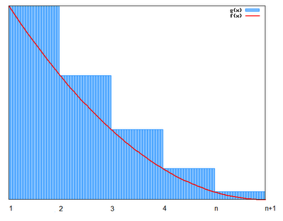
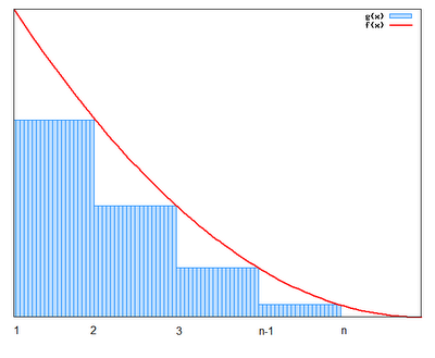
(2) Using the Integral Test (see Theorem 1, here),

We know that if ∑ (1/n^s) converges, then ∫ (1,∞) 1/x^sdx also converges.

(3) If we define a function so that f(x) = 1/ceiling(x)^s, we can conclude that ∫ (1,∞) 1/x^s is less than ∫ (1,∞) 1/ceiling(x)^s = ∑ (n=1,∞) 1/n^s which is less than 1 + ∫ (1,∞) 1/x^sdx since:

(a) ∫ (1,∞) 1/x^s is less than ∫ (1,∞) 1/ceiling(x)^s

At each point x ≤ ceiling(x) so that at each point x^s ≤ ceiling(x)^s.



(b) ∫ (1,∞) 1/ceiling(x)^s = ∑ (n=1,∞) 1/n^s

This follows from the fact that for each interval, ∫ (x,x+1) 1/ceiling(x)^s= ∑(n=x,x) 1/n^s.

(c) ∑ (n=1,∞) 1/n^s is less than 1 + ∫ (1,∞) 1/x^sdx

This follows since ∑ (n=1,∞) 1/n^s - 1 is less than ∫ (1,∞) 1/x^sdx and therefore ∑ (n=1,∞) 1/n^s is less than 1 + ∫ (1,∞) 1/x^sdx.



(4) ∫ (1,∞) 1/x^sdx = 1/(s-1)

(a) ∫ (1,∞) 1/x^sdx = lim (t → ∞) ∫ (1,t) 1/t^sdt

(b) ∫ 1/t^sdt = ∫ t^-s dt = 1/(-s+1) (t^-s+1) + C = -1/(s-1)(1/t^s-1) + C [See here for review of integral if needed]

(c) lim (t → ∞) ∫ (1,t) 1/t^sdt = lim(t → ∞) ( [-1/(s-1)][1/t^s-1] + [1/(s-1)]*[1/1^s-1])=

= lim (t → ∞) [(-1)/[(s-1)*(t^s-1)] + [1/(s-1)]*1]

(d) As t → ∞, 1/t → 0 so we get:

= [0*(-1)/(s-1)] + [1/(s-1)] = 1/(s-1)

(5) This gives us that:

1/(s-1) is less than ζ(s) is less than 1 + 1/(s-1)

(6) Multiplying (s-1) to all sides, gives us:

1 is less than (s-1)*ζ(s) is less than (s-1) + 1 = s

(7) Now as s goes to 1, it is clear that we have:

1 ≤ (s-1)*ζ(s) ≤ 1.

(8) Using the Squeeze Law (see Lemma 3, here), we can conclude that the limit is 1.

QED

References

• Harold M. Edwards, Fermat's Last Theorem: A Genetic Introduction, Springer, 2000.
  

Euler Product Formula Converges for Re(s) > 1

To move ahead on Kummer's class number formula for ideal numbers, it is necessary to review the proof for the convergence of Euler's Product Formula, that is:

∑ n^-s = ∏ (1 - p^-s)^-1

Ernst Kummer proposed an equivalent formula for ideal numbers which I will talk about in a future blog. If you are not familiar with the notation Re(s), start here.

Theorem 1: For s greater than 1, ∑ (n=1, ∞) n^-s converges absolutely.

Proof:

(1) Let σ = Re(s)

(2) abs(n^-s) = n^-σ [See Theorem, here]

(3) Let M be any integer ≥ 1.

(4) Let N be any integer greater than M

(5) Using the triangle inequality for complex numbers (See Lemma 3, here for more details) abs[∑ (n=M+1,N) n^-s)]≤ ∑ (n=M+1,N) abs(n^-s) = ∑ (n=M+1,N) n^-σ

(6) From a previous result (See Corollary 1.2, here for more details), we know that ∑ (n=M+1,N) n^-σ converges.

*(6) Since f(x)=1/x^s is positive, continuous, and decreasing for x ≥ 1, I can use a result from an earlier blog (See Corollary 1.2, here for more details) to establish that ∑ (n=M+1,N) n^-σ converges.

(7) Since all n^-s ≥ 0, we can see that it converges absolutely. [See here for definition and properties of absolute convergence]

QED

Theorem 2: For S greater than 1, ∏(1 - p^-s) converges absolutely

Proof:

(1) ∑ abs(p^-s) = ∑(p^-σ) where σ = Re(s). [See Theorem 2, here for proof]

(2) ∑(p^-σ) ≤ ∑(n^-σ) and since ∑ (n^-σ) is convergent (by Theorem 1 above), ∑ abs(p^-s) is also convergent.

(4) ∑ abs(p^-s) is convergent implies that ∏ (1 - p^-s) is convergent. [See Lemma 6, here]

(5) And this means that ∏ (1 - p^-s)^-1 is also convergent. [See Lemma 6, here]

(6) Since ∑ abs(p^-s) is convergent, it follows that ∏(1 - p^-s) is absolutely convergent and therefore ∏ (1 - p^-s)^-1 is absolutely convergent since:

(a) Assume ∑ abs(p^-s) is convergent

(b) It follows that ∏(1 - abs[p^-s]) is convergent [See Lemma 3, here]

(c) Which means that ∏(1 - p^-s) is absolutely convergent. [See Definition 1, here]

(d) Using the Reciprocal Property of limits (see Lemma 6, here), we can see that 1/∏(1 - abs[p^-s]) is also convergent.

(e) Using the definition of absolute convergence for infinite products (see step #6c above), we see that ∏ (1 - p^-s)^-1 absolutely convergent.

QED

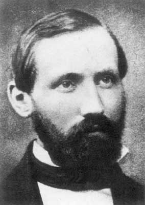
Bernhard Riemann

Bernhard Riemann was born in the Kingdom of Hanover (now, Germany) on September 17, 1826. He was the second of six children. He was home schooled by his father, Lutheran minister, until he was 10. Through out his life, he remained very close to his family and very religious.

When he was 14, Riemann moved in with his grandmother and attended school in Lyceum. He entered the gymnasium in Luneburg in 1842. At the gymnasium, Riemann showed strong interest in mathematics. It is said that he read a 900 page book by Adrien Legendre on number theory in 6 days.

In 1846, Riemann enrolled in theology at the University of Gottingen. He continued to take classes in mathematics and later, after consulting with his father, changes his focus from theology to mathematics. At Gottingen, he was able to takes courses from the legendary mathematician Carl Friedrich Gauss.

Despite having Gauss on its faculty, the University of Gottingen was, at this time, secondary in mathematics to the University of Berlin. Riemann transferred there in 1847 and was able to attend courses in advanced mathematics given by Jakob Steiner, Carl Jacobi, Johann Dirichlet, and Ferdinand Eisenstein. These were exciting times for Riemann and he became particularly influenced by the theories of Dirichlet. It is said that at this time, Riemann built up what would become his general theory of complex variables.

Riemann returned to the University of Gottingein in 1849 to work on his Ph.D. thesis under the guidance of Gauss. Riemann was also greatly influenced by Wilhem Weber in theoretical physics and Johann Listing in topology.

Riemann's thesis was on what are today known as Riemann surfaces. In this groundbreaking work, Riemann used topology to analyze complex variables. The MacTutor biography describes this work as: "a strikingly original piece of work which examined the geometric properties of analytic functions, conformal mappings, and the connectivity of surfaces."

Today, Riemann's Ph.D. thesis is considered to be one of the most impressive that has ever been produced. Based on Gauss's recommendation, Riemann was offered a post at the University of Gottingen as a lecturer. To become a lecturer, he needed to achieve a post-doctoral degree called a Habilitation. To complete this degree, he needed to make a presentation on an advanced topic. He proposed three topics to Gauss and to his surprise, Gauss selected geometry. So, on June 10, 1854, Riemann presented a lecture on what is today known as Riemannian geometry which would later be the basis of Einstein's general theory of relativity. The lecture is today considered a classic.

The story goes that Riemann's lecture was so advanced for its time that only Gauss appreciated the depths of the ideas. While the other technical members of the audience listened politely, Gauss was greatly excited. The MacTutor biography quotes an eyewitness: "The lecture exceeded all his [Gauss's] expectations and greatly surprised him. Returning to the faculty meet, he [Gauss] spoke with the greatest phrase and rare enthusiasm to Wilhelm Weber about the depth of the thoughts that Riemann had presented."

When Gauss died in 1855, his replacement was Johann Dirichlet. In 1857, Riemann became a professor of mathematics. At this time, he wrote a paper on the theory of abelian functions. At the same time, Karl Weierstrass was working on the same topic. Riemann's paper was very advanced. Felix Klein writes: "It [Riemann's paper] contained so many unexpected, new concepts that Weierstrass withdrew his paper and in fact published no more."

In 1859, Dirichlet died and Riemann replaced him as the chair of mathematics. He was also admitted to the the Berlin Academy of Sciences. His nomination read (from MacTutor):

Prior to the appearance of his most recent work [Theory of abelian functions], Riemann was almost unknown to mathematicians. This circumstance excuses somewhat the necessity of a more detailed examination of his works as a basis of our presentation. We considered it our duty to turn the attention of the Academy to our colleague whom we recommend not as a young talent which gives great hope, but rather as a fully mature and independent investigator in our area of science, whose progress he in significant measure has promoted.

As a newly elected member of the Academy of Sciences, Riemann was expected to make a techincal presentation. Riemann's presentation unleashed what is today known as the Riemann Hypothesis. This is the most famous and most important open problem in number theory. It was identified by David Hilbert among his famous collection of 23 mathematical problems. The purpose of the paper was to outline a method for determining the number primes less than a given number.

At 36, he married Elise Koch and it seemed like his mathematical impact was only just beginning. Unfortunately, around this time, he got sick with what would later turn out to be tuberculosis. He continued to travel to Italy where he hoped a warmer environment would help his health and then returned to Gottingen. He died on July 20, 1866 in Italy.

Over all, Riemann's output was small but the influence of that output makes him one of the most influential mathematicians of the nineteenth century. He masterfully combined topics of topology, geometry, analysis, and number theory to show how each complemented the other areas. His impact on such a wide range of topics makes him one of the most important mathematicians of all time.

References

• "Bernhard Riemann", the MacTutor Biography
• John Derbyshire, Prime Obsession, Plume, 2004
  

Bernoulli Numbers and the Riemann Zeta Function

Leonhard Euler used the Bernoulli numbers to generalize his solution to the Basel Problem. This is the problem that put Euler on the map mathematically.

The Bernoulli numbers are named after Jacob Bernoulli, the same Bernoulli who popularized the Basel Problem that Euler solved. Bernoulli had been unable to solve the Basel Problem but Euler later showed how the numbers he had identified could be used to provide a general solution to ζ(2s) = ∑ n^-2s = 1/1^2s + 1/2^2s + ...

The content in today's blog is taken straight from Graham, Knuth, Patashnik's Concrete Mathematics.

The following are definitions for the hyperbolic functions. For those who would like a background on them, see here.

Definition 1: sinh z

sin h z = (e^z - e^-z)/2

Definition 2: cosh z

cosh z = (e^z + e^-z)/2

Definition 3: coth z

coth z = (cosh z)/(sinh z)

Now, we use these definitions in this lemma.

Lemma 1: z/(e^z - 1) + (z/2) = (z/2) coth (z/2)

Proof:

(1) z/(e^z - 1) + (z/2) = (2z + z[e^z - 1])/(2[e^z-1]) = (2z -z + z[e^z])/(2[e^z-1]) = (z/2)(e^z+1)/(e^{z - 1})

(2) (z/2)(e^z + 1)/(e^z-1) = [e^-(z/2)/e^-(z/2)]* (z/2)(e^z + 1)/(e^z-1) =

= (z/2)[(e^z/2 + e^-z/2)/(e^z/2 - e^-z/2)] =

= (z/2) coth (z/2)

QED

Corollary 1.1: z coth z = ∑ (n ≥ 0) 4ⁿB_2n(z²ⁿ)/(2n!)

Proof:

(1) From Lemma 1 above:

z/(e^z - 1) + (z/2) = (z/2) coth (z/2)

(2) Using a previous result (see Corollary, here), we also know that:

z/[e^z - 1] + (z/2) = ∑ (n ≥ 0)B_2nz⁽²ⁿ⁾/(2n)!

(3) Subsituting 2z for z gives us:

(2z)/(e^2z - 1) + z = z coth z = ∑ (n ≥ 0)B_2n(2z)⁽²ⁿ⁾/(2n)! =

= ∑ (n ≥ 1)(4)ⁿB_2n(z)⁽²ⁿ⁾/(2n)!

QED

Lemma 2: cot x = i coth ix

Proof:

(1) e^ix = i sin x + cos x [See Euler's Formula Theorem, here]

(2) cosh ix = (e^ix + e^-ix)/2 = (isinx + cos x + isin(-x) + cos(-x))/2 = 2cos(x)/2 = cos(x)

(3) sinh ix = (e^ix - e^-ix)/2 = (isin x + cos x - isin(-x) -cos(-x))/2 = 2isin(x)/2 = isin(x)

(4) i coth ix = i (cosh(ix)/sinh(ix)) = i ( cos(x)/isin(x)) = cot(x)

QED

Lemma 3: z cot z = ∑ (n ≥ 0) (-4)ⁿB_2n(z²ⁿ)/(2n)!

where B_i is a Bernoulli number [See Definition 1, here for definition of Bernoulli numbers]

Proof:

(1) From Corollary 1.1 above, we have:

z coth z = ∑ (n ≥ 0)B_2n(2z)⁽²ⁿ⁾/(2n)!

(2) Using Lemma 2 above, we have:

z cot z = ∑ (n ≥ 0)B_2n(2iz)⁽²ⁿ⁾/(2n)! =

= ∑ (n ≥ 1)(-4)ⁿB_2n(z)⁽²ⁿ⁾/(2n)!

QED

Lemma 4: cot z = (1/2ⁿ) ∑ (k=0, 2ⁿ-1) cot ([z + kπ]/2ⁿ)

Proof:

(1) I will use induction for this proof.

(2) For n=1, we have:

cot z = (1/2) cot(z/2) + (1/2) cot(z/2 + π/2)

(a) Since cot(z/2 + π/2) = - tan(z/2) [See Corollary 1.6, here], we have:

(1/2)cot(z/2) + (1/2)cot(z/2 + π/2) = (1/2)[cot(z/2) - tan(z/2)] = (1/2)[cos(z/2)/sin(z/2) - sin(z/2)/cos(z/2)] = (1/2)[cos²(z/2) - sin²(z/2)]/[sin(z/2)cos(z/2)]

(b) Since cos(z) = cos²(z/2) - sin²(z/2) [see Lemma 3, here], we have:

cot z = (1/2)[cos(z)]/[sin(z/2)cos(z/2)]

(c) Since sin(2x) = 2sin(x)cos(x) [See Lemma 2, here], we have:

cot z = (1/2)[cos(z)/[(1/2)sin(z)]] = cos(z)/sin(z) = cot z

(3) Assume that cot z = (1/2ⁿ) ∑ (k=0, 2ⁿ-1) cot ([z + kπ]/2ⁿ) for n ≥ 1.

(4) Using cot(2x) = (1/2)[cot(x) - tan(x)] [See Corollary 3.6, here], we have:

cot z = (1/2ⁿ) ∑ (k=0, 2ⁿ-1) cot ([z + kπ]/2ⁿ) =

= (1/2ⁿ⁺¹) ∑ (k=0,2ⁿ-1) [ cot([z + kπ]/2ⁿ⁺¹) - tan(z + kπ]/2ⁿ⁺¹) ]

(5) Since -tan(x) = cot(x + π/2), we have:

cot z = (1/2ⁿ⁺¹) ∑ (k=0,2ⁿ-1) [ cot([z + kπ]/2ⁿ⁺¹) + cot(z + kπ]/2ⁿ⁺¹ + π/2) ] =

(1/2ⁿ⁺¹) ∑ (k=0,2ⁿ-1) [ cot([z + kπ]/2ⁿ⁺¹) + cot(z + (k+ 2ⁿ)π]/2ⁿ⁺¹) ] =

(1/2ⁿ⁺¹) ∑ (k=0,2ⁿ-1) cot([z + kπ]/2ⁿ⁺¹) + (1/2ⁿ⁺¹) ∑ (k=0,2ⁿ-1) cot([z + (k + 2ⁿ)π]/2ⁿ⁺¹) =

= (1/2ⁿ⁺¹) ∑ (k=0,2ⁿ-1) cot([z + kπ]/2ⁿ⁺¹) + (1/2ⁿ⁺¹) ∑ (k=2ⁿ,2ⁿ⁺¹-1) cot([z + kπ]/2ⁿ⁺¹) =

= (1/2ⁿ⁺¹) ∑ (k=0, 2ⁿ⁺¹-1) cot ([z + kπ]/2ⁿ⁺¹)

QED

Corollary 4.1: cot z = (1/2ⁿ) cot (z/2ⁿ) - (1/2ⁿ) tan (z/2ⁿ) + ∑ (k=1, 2^n-1-1) (1/2ⁿ) (cot[(z + kπ)/2ⁿ] + cot[(z - kπ)/2ⁿ])

Proof:

(1) From Lemma 4, substituting (n-1) for (n), we get:

cot z = (1/2^n-1) ∑ (k=0, 2^n-1-1) cot ([z + kπ]/2^n-1) =

= (1/2^n-1) cot(z/2^n-1) + (1/2^n-1) ∑ (k=1, 2^n-1-1) cot([z + kπ]/2^n-1)

(2) Using cot(2x) = (1/2)[cot(x) - tan(x)] (see Corollary 3.6, here), we get:

(1/2^n-1) cot(z/2^n-1) = (1/2ⁿ)[cot(z/2ⁿ) - tan(z/2ⁿ)]

(3) We also get:

(1/2^n-1) ∑ (k=1, 2^n-1-1) cot([z + kπ]/2^n-1) = (1/2ⁿ) ∑ (k=1, 2^n-1-1) [cot([z + kπ]/2ⁿ) - tan([z+kπ]/2ⁿ)]

(4) To complete the proof, we just need to show that ∑ (k=1, 2^n-1-1) -tan([z+kπ]/2ⁿ) = ∑ (k=1, 2^n-1-1) cot([z - kπ]/2ⁿ)

(5) First, we note that -tan(z) = cot(z - π/2) since:

-tan(z) = cot(z + π/2) = cot(z - π + π/2) = cot(z - π/2) [See Corolary 1.6 and Corollary 1.5, here]

(6) This gives us that:

∑ (k=1, 2^n-1-1) -tan([z + kπ]/2ⁿ) = ∑(k=1,2^n-1-1) cot([z + kπ]/2ⁿ - π/2) =

= ∑ (k=1,2^n-1-1) cot([z + (-2^n-1 + k)π]/2ⁿ)

(7) Now we can see that -2^n-1 + k = -1 when k=2^n-1-1 and -2^n-1 + k = -2^n-1+1 when k = 1.

(8) Therefore:

∑ (k=1,2^n-1-1) cot([z + (-2^n-1 + k)π]/2ⁿ) = ∑ (k=1,2^n-1-1) cot([z - kπ]/2ⁿ)

QED

Lemma 5: lim (z → 0) z cot z = 1

Proof:

(1) lim(z → 0) z cot z = lim(z → 0) cos(z)* lim(z → 0) (z/sin(z)) [By Product Rule for Limits, see Lemma 2, here]

(2) lim(z → 0) cos(z) = 1 [See Property 6, here if needed]

(3) lim (z → 0) (z/sin(z)) = lim(z → 0) 1/(sin(z)/z) [By the Reciprocal Law for Limits, see Lemma 6 here]

(4) lim (z → 0) (sin(z)/z) = 1 [See Lemma 2, here]

(5) Putting it all together gives us:

lim (z → 0) z cot z = lim(z → 0) cos(z) * 1/[lim(z → 0) sin(z)/z] = 1*(1/1) = 1

QED

Corollary 5.1: z cot z = 1 - 2 ∑ (k ≥ 1) z²/[k²π² - z²]

Proof:

(1) Using Corollary 4.1 above, we have:

z cot z = (z/2ⁿ) cot (z/2ⁿ) - (z/2ⁿ) tan (z/2ⁿ) + ∑ (k=1, 2^n-1-1) (z/2ⁿ) (cot[(z + kπ)/2ⁿ] + cot[(z - kπ)/2ⁿ])

(2) Since n can take any value, we can see that:

z cot z = lim (n → ∞) [ (z/2ⁿ) cot (z/2ⁿ) - (z/2ⁿ) tan (z/2ⁿ) + ∑ (k=1, 2^n-1-1) (z/2ⁿ) (cot[(z + kπ)/2ⁿ] + cot[(z - kπ)/2ⁿ]) ]

(3) As n approaches ∞, z/2ⁿ approaches 0, so that using Lemma 5 above we have:

lim(n → ∞) (z/2ⁿ)cot(z/2ⁿ) = lim (z → 0) (z) cot(z) = 1

(4) Likewise,

lim(n → ∞) -(z/2ⁿ)tan(z/2ⁿ) = lim(z → 0) -z*tan(z) = lim(z → 0) (-z) * sin(z)/cos(z) = (-z)*(0)*(1) = 0 [See Product Rule for Limits for details if needed, see Lemma 2, here]

(5) Now, (z/2ⁿ) = [(z + kπ)/2ⁿ]*[z/(z + kπ)] so that:

lim(n → ∞) (z/2ⁿ)*cot([z + kπ]/2ⁿ) =

lim(n → ∞) [z/(z + kπ)]*[(z+kπ)/2ⁿ]*cot([z + kπ]/2ⁿ)

(6) Let u = (z + kπ)/2ⁿ

(7) As n → ∞, u → 0, so that we have:

lim(n → ∞) (z/2ⁿ)*cot([z + kπ]/2ⁿ) =
lim(u → 0) [z/(z + kπ)]*u*cot(u) = [z/(z + kπ)]*1 = z/(z + kπ)

(8) Let v = (z - kπ)/2ⁿ

(9) As n → ∞, v → 0, so that we have:

lim(n → ∞) (z/2ⁿ)*cot([z - kπ]/2ⁿ) =
lim(v → 0) [z/(z - kπ)]*v*cot(v) = [z/(z - kπ)]*1 = z/(z - kπ)

(10) So, lim (n → ∞) [ (z/2ⁿ)cot([z + kπ]/2ⁿ) + (z/2ⁿ)cot([z - kπ]/2ⁿ) = z/(z + kπ) + z/(z - kπ) = [z*(z - kπ) + z(z + kπ)]/(z² - k²π²) = (2z²)/(z² - k²π²) [See Addition Rule for Limits, see Corollary 8.1, here]

(11) Finally,

lim (n → ∞) (z/2ⁿ) cot (z/2ⁿ) - (z/2ⁿ) tan (z/2ⁿ) + ∑ (k=1, 2^n-1-1) (z/2ⁿ) (cot[(z + kπ)/2ⁿ] + cot[(z - kπ)/2ⁿ]) =

= 1 - 0 + ∑(k ≥ 1) 2z²/(z² - k²π²) = 1 - 2*∑ (k ≥ 1) z²/(k²π² - z²)

QED

Lemma 6: z²/[k²π² - z²] = ∑ (i ≥ 1) z²ⁱ/[k²ⁱπ²ⁱ]

Proof:

(1) 1/(1 - x) = 1 + x + x² + ... [See Lemma 1, here]

(2) x/(1 - x) = x + x² + x³ + ...

(3) Let x = (z²)/(k²π²)

(4) Then:

[(z²)/(k²π²)]/[1 - (z²)/(k²π²)] =

(z²)/[(k²π²](1 - (z²)/(k²π²)] =

= z²/(k²π² - z²)

QED

Theorem: ζ(2n) = (-1)^n-1[2^2n-1π²ⁿB_2n]/(2n)!

where:

ζ(s) = 1/1^s + 1/2^s + 1/3^s + ...

B_i is a Bernoulli number

Proof:

(1) z cot z = 1 - 2 ∑ (k ≥ 1) z²/[k²π² - z²] [See Lemma 5 above]

(2) Using Lemma 6 above, we have:

z cot z = 1 - 2∑ (k ≥ 1)[ z²/k²π² + z⁴/k⁴π⁴ + z⁶/k⁶π⁶ + ... ]

(3) Since for each of term of this sum, k can take all integer values ≥ 1, we replace the ∑(k ≥ 1) with:

z cot z = 1 - 2(z²ζ(2)/π² + z⁴ζ(4)/π⁴ + z⁶ζ(6)/π⁶ + ...

(4) From Lemma 3 above, we have:

z cot z = ∑ (n ≥ 0) (-4)ⁿB_2n(z²ⁿ)/(2n)! = B₀ + ∑ (n ≥ 1) (-4)ⁿB_2n(z²ⁿ)/(2n)! =
= 1 + ∑ (n ≥ 1) (-4)ⁿB_2n(z²ⁿ)/(2n)!

(5) Equating the equations in step #3 and step #4 gives us:

- 2(z²ζ(2)/π² + z⁴ζ(4)/π⁴ + z⁶ζ(6)/π⁶ + ... = ∑ (n ≥ 1) (-4)ⁿB_2n(z²ⁿ)/(2n)!

(6) This gives us for each term i ≥ 1:

-2z^2*iζ(2*i)/π^2*i = (-4)ⁱB_2i(z²ⁱ)/(2i)!

(7) Solving for ζ(2*i), this gives us:

ζ(2i) = (-4)ⁱB_2iπ²ⁱ/[(2i)!(-2)] =

= (-1)^i-1(2^2i-1π²ⁱB_2i)/(2i)!

QED

Bernoulli Polynomials

In today's blog, I introduce Bernoulli polynomials and show how they can be used to present an even shorter version of the summation formula we found for Bernoulli numbers.

The content in today's blog is taken from Concrete Mathematics (Graham, Knuth, and Patashnik, 1989).

Definition 1: Bernoulli Polynomial



where n ≥ 0 and b_k is the Bernoulli number (see Definition 1, here)

I will now show how Bernoulli Polynomials can be used to create a concise summation formula.

Lemma 1: ∑ (k=0,n) e^kz = [e^nz - 1]/[e^z - 1]

Proof:

(1) Let S_n = ∑ (k=0,n-1) e^kz = ∑ (k=0, n) (e^z)^k = e⁰ + e^z + e^2z + ... + e^(n-1)z

(2) S_n + (e^z)ⁿ = (e^z)⁰ + ∑ (k=0,n-1) (e^z)^k+1

(3) (e^z)S_n = (e^z)∑ (k=0,n-1) (e^z)^k = ∑ (k=0,n) (e^z)^k+1

(4) Putting #2 and #3 together gives us:

S_n + (e^z)ⁿ = (e^z)S_n + 1

(5) So, solving for S_n gives us:

S_n - (e^z)S_n = 1 - (e^z)ⁿ = S_n(1 - e^z)

(6) Dividing both sides by (1 - e^z) gives us:

S_n = [1 - (e^z)ⁿ]/[1 - e^z] *(-1)/(-1) = [e^nz - 1]/[e^z - 1]

QED

NOTE: If you are not familiar with the idea of generating functions, start here.

Corollary 1.1: Generating Function for Bernoulli Polynomials

∑ (m ≥ 0) B_m(n)z^m/m! = (ze^xz)/(e^z - 1)

Proof:

(1) Let T(z,n) be the generating function for Bernoulli polynomials B_m(n) so that we have:

T(z,n) = B₀(n)z⁰/0! + B₁(n)z¹/1! + .... = ∑ (m=0,∞) B_m(n)z^m/m!

(2) Inserting the definition for Bernoulli polynomials (see Definition1 above), we have:

T(z,n) = ∑ (m=0,∞) ∑(k=0; m) [(m!/[k!][m-k]!)*B_kx^n-k] z^m/m!

(3) Using a previous result on binomial convolution (see Lemma 1, here), we can reverse this to get:
∑(m=0; ∞) ∑(k=0;m) [(m!/[k!][m-k]!)*B_kx^n-k] z^m/m! = [∑(m=0; ∞) B_mz^m/m!]*[∑(m=0, ∞) x^mz^m/m!]

(4) From a previous result (see Theorem, here), we have:

∑ (m ≥ 0) (B_m)z^m/m! = z/[e^z - 1]

(5) Further, using the power series for e (see Lemma 2, here), we have:

e^xz = ∑ (m ≥ 0) x^mzm/m!

(6) Inserting these results gives us:

T(z,n) = ∑(m=0; ∞) ∑(k=0;m) [(m!/[k!][m-k]!)*B_kx^n-k] z^m/m! = [∑(m=0; ∞) B_mz^m/m!]*[∑(m=0, ∞) x^mz^m/m!] =

= (z/[e^z - 1])*(e^xz) = (ze^xz)/(e^z - 1)

QED

Theorem: S_m-1(n) = (1/m)(B_m(n) - B_n(0))

Proof:

(1) S_m(n) = 0^m + 1^m + ... + (n-1)^m = ∑ (k=0,n) k^m [See Definition2, here for definition of S_m(n)]

(2) Let S(z) = ∑ (m ≥ 0) S_m(n) z^m = S₀(n) + S₁(n)z + S₂(n)z² + ... = ∑ (m ≥ 0) ∑ (k=0,n) k^mz^m

(3) Using the power series for e^z (see Lemma 2, here), we know that:

e^z = ∑ (n ≥ 0) zⁿ/n! = z⁰/0! + z¹/1! + ... + zⁿ/n!

(4) We can see that:

e^kz = ∑ (m ≥ 0) (kz)^m/m! = ∑(m ≥ 0)k^mz^m/m!

(5) Let G(z,n) be the generating function for S(z) so that we have:

G(z,n) = S₀(n)x⁰/0! + S₁(n)z¹/1! + S₂(n)/z²/2! + ... = ∑ (m ≥ 0) S_m(n)z^m/m!

(6) Using step #2, then we have:

G(z,n) = ∑ (m ≥ 0) ∑ (k=0, n) k^mz^m/m! = ∑ (k=0,n) e^kz

(7) Using the Lemma 1 above, we have:

G(z,n) = [e^nz - 1]/[e^z - 1]

(8) Let T(z,n) be the generating function for the Bernoulli Polynomial

(9) Using Corollary 1.1 above, we have:

T(z,n) = ∑ (m ≥ 0) B_m(n)z^m/m! = (ze^xz)/(e^z - 1)

(10) This then gives us that:

T(z,n) - T(z,0) = (ze^nz)/(e^z - 1) - (ze^0z)/(e^z - 1) = z[e^nz - 1]/[e^z-1]

(11) This shows that z*G(z,n) = [T(z,n) - T(z,0)]

(12) So that we have:

S₀(n)z¹/0! + S₁(n)z²/1! + S₂(n)/z³/2! + ... = [(B₀(n)z⁰/0! + B₁(n)z¹/1! + ....) - (B₀(0)z⁰/0! + B₁(0)z¹/1! + ....)]

(13) Lining up, equal powers of zⁱ gives us:

S_m-1(n)/(m-1)! = B_m(n)/m!] - B_m(0) /m!

(14) Multiplying both sides by (m-1)! gives us:

S_m-1(n) = (1/m)[B_m(n) - B_m(0)]

<sub>QED

References</sub>

• "Bernoulli Polynomials", Wikipedia.com
• Ronald L. Graham, Donald E. Knuth, Oren Patashnik, Concrete Mathematics, Addison-Wesley, 1989

A Generating Function for the Bernoulli Numbers

In my previous blog, I defined the Bernoulli numbers using a recurrence relation:

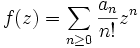
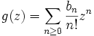
In today's blog, I will show how the Bernoulli numbers can be used with a generating function. A generating function is a power series, that is, a compact expression that defines an infinite sum. For background on generating functions, I recommend the wikipedia article (see reference) or Graham et al's Concrete Mathematics (see reference).

The content in today's blog is taken from Concrete Mathematics. The term "binomial convolution" is taken from this work. A "convolution" is the multiplication of two generating functions. This lemma is called a "binomial convolution" by Graham et al because the result involves binomial coefficients (see binomial theorem, here, for more details).

Lemma 1: Binomial Convolution

Let:





h(z) = f(z)*g(z)

Then there exists d_n such that:



with:



Proof:

(1) Multiplying f(z) with g(z) gives us:



(2) Grouping the result by zⁱ gives us:



(3) If we set c_i to each coefficient. For example, if we set c₀ to (a₀b₀)/(0!0!), then we have the following formula:



(4) Now, let's define a value d_i such that:



(5) This then gives us that:
d_i/(i!) = c_i


(6) Combining step #5 with step #2 and step #3 gives us:



QED

Thereom: Generating Function for the Bernoulli Numbers

z/(e^z - 1) is the generating function for the Bernoulli numbers

Proof:

(1) Let G(z) = ∑ (n ≥ 0) B_nzⁿ/n! where B_i is the Bernoulli number for i.

(2) We know from a previous result (see Lemma 2, here) that:

e^z = ∑ (n ≥ 0) zⁿ/n!

(3) So we can use Lemma 1 above to show that:



(4) Now, the definition for Bernoulli numbers (see Definition 1, here) is:



for all cases except for B₀ where B₀ = 1.

(5) If we let n=m+1 and add B_n to both sides, then we have:



or B_n + 1 in the case where n=m+1=1.

(6) This enables us to simplify the result in step #3 to get:



Note: the z at the bottom comes from the fact that at n=1, our result is (B₁+1)z¹/1! = B₁z¹/1! + z.

(7) If we subtract G(z) from both sides, we get:

(e^z)G(z) - G(z) = z =

G(z)(e^z - 1) = z

(8) Dividing both sides by e^z - 1 gives us:

G(z) = z/(e^z - 1)

QED

Corollary: B_2i+1=0 if i ≥ 1.

Proof:

(1) z/(e^z - 1) = ∑ (n ≥ 0) B_nzⁿ/n! [This follows from the theorem above]

(2) Now, B₁ = -(1/2) [See Definition 1, here]

(3) So,

z/(e^z - 1) + (z/2) = ∑ (n ≥ 0 and n ≠ 1) B_nzⁿ/n!

We subtract (-z/2) instead of -1/2 because we are removing this item from a generating function where each value in the sum z/(e^z-1) pairs up with a unique term of the sum.

In this case, B₁ matches up with the term B₁(z¹)/1! which equals -z/2.

(4) z/(e^z - 1) + (z/2) = (2z + z[e^z - 1])/(2[e^z-1]) = (2z -z + z[e^z])/(2[e^z-1]) =

= (z/2)(e^z+1)/(e^{z - 1})

(5) (z/2)(e^z + 1)/(e^z-1) = [e^-(z/2)/e^-(z/2)]* (z/2)(e^z + 1)/(e^z-1) =

= (z/2)[(e^z/2 + e^-z/2)/(e^z/2 - e^-z/2)]

(6) So, we see in step #5, that if we replace z with (-z), the identity remains unchanged.

(-z/2)[(e^-z/2 + e^-(-z/2)]/(e^-z/2 - e^-(-z)/2) =

= -z/2[e^-z/2 + e^z/2]/(e^-z/2 - e^z/2) =

= z/2[e^z/2 + e-z/2]/(e^z/2 - e^-z/2)

In the language of mathematics, a function is called even if f(-x)=f(x) and we call a function odd if f(-x) = -f(x). [See here for more details]

Example: cos(x) is an even function while sin(x) is an odd function. [See here for review of sin and cos]

(7) But this means that the same must hold true for ∑ (n ≥ 0 and n ≠ 1) B_nzⁿ/n!

Since by Step #3, we showed that they are equal functions.

So that we have:

∑ (n ≥ 0 and n ≠ 1) B_nzⁿ/n! = ∑ (n ≥ 0 and n ≠ 1) B_n(-z)ⁿ/n! = ∑ (n ≥ 0 and n ≠ 1) (-1)ⁿ(B_nzⁿ/n!)

(8) Matching up each of the terms according to powers of zⁿ, this gives us that:

B_n = (-1)ⁿB_n

(9) But this can only be true if B_n = 0 when n is odd.

QED

References

• "Generating Function," Wikipedia.com
• Ronald L. Graham, Donald E. Knuth, Oren Patashnik, Concrete Mathematics, Addison-Wesley, 1989
• "Odd Bernoulli Numbers are 0", PlanetMath.org
• "Even and Odd Functions", Wikipedia.com

References

Saturday, November 11, 2006
Monday, November 06, 2006
Sunday, October 29, 2006
Monday, October 23, 2006